import os
import h5py
import numpy as np
import pandas as pd
import geopandas as gp
from shapely.geometry import Point
import geoviews as gv
from geoviews import opts, tile_sources as gvts
import holoviews as hv
gv.extension('bokeh', 'matplotlib')
The Global Ecosystem Dynamics Investigation (GEDI) mission aims to characterize ecosystem structure and dynamics to enable radically improved quantification and understanding of the Earth's carbon cycle and biodiversity. The GEDI instrument produces high resolution laser ranging observations of the 3-dimensional structure of the Earth. GEDI is attached to the International Space Station and collects data globally between 51.6$^{o}$ N and 51.6$^{o}$ S latitudes at the highest resolution and densest sampling of any light detection and ranging (lidar) instrument in orbit to date. The Land Processes Distributed Active Archive Center (LP DAAC) distributes the GEDI Level 1 and Level 2 products. The L1B and L2 GEDI products are archived and distributed in the HDF-EOS5 file format.
This tutorial was developed using an example use case for a project being completed by the National Park Service. The goal of the project is to use GEDI L1B data to observe GEDI waveforms over Redwood National Park in northern California.
This tutorial will show how to use Python to open GEDI L1B files, visualize the full orbit of GEDI points (shots), subset to a region of interest, visualize GEDI full waveforms, and export subsets of GEDI science dataset (SDS) layers as GeoJSON files that can be loaded into GIS and/or Remote Sensing software programs.
It is recommended to use Conda, an environment manager to set up a compatible Python environment. Download Conda for your OS here: https://www.anaconda.com/download/. Once you have Conda installed, Follow the instructions below to successfully setup a Python environment on Linux, MacOS, or Windows.
This Python Jupyter Notebook tutorial has been tested using Python version 3.7. Conda was used to create the python environment.
Using your preferred command line interface (command prompt, terminal, cmder, etc.) type the following to successfully create a compatible python environment:
conda create -n geditutorial -c conda-forge --yes python=3.7 h5py shapely geopandas pandas geoviews holoviews
conda activate geditutorial
jupyter notebook
If you do not have jupyter notebook installed, you may need to run:
conda install jupyter notebook
If you prefer to not install Conda, the same setup and dependencies can be achieved by using another package manager such as pip.
This tutorial uses the GEDI L1B observation from June 19, 2019 (orbit 02932). Use the link below to download the file directly from the LP DAAC Data Pool:
The repository containing all of the required files is located at: https://git.earthdata.nasa.gov/projects/LPDUR/repos/gedi-tutorials/browse
import os
import h5py
import numpy as np
import pandas as pd
import geopandas as gp
from shapely.geometry import Point
import geoviews as gv
from geoviews import opts, tile_sources as gvts
import holoviews as hv
gv.extension('bokeh', 'matplotlib')
inDir = os.getcwd() + os.sep # Set input directory to the current working directory
inDir defined above. You will need to download the file directly from the LP DAAC Data Pool in order to execute this tutorial.¶inDir directory defined above.gediFiles = [g for g in os.listdir() if g.startswith('GEDI01_B') and g.endswith('.h5')] # List all GEDI L1B .h5 files in inDir
gediFiles
['GEDI01_B_2019170155833_O02932_T02267_02_003_01.h5']
L1B = 'GEDI01_B_2019170155833_O02932_T02267_02_003_01.h5'
L1B
'GEDI01_B_2019170155833_O02932_T02267_02_003_01.h5'
GEDI01_B: Product Short Name
2019170155833: Julian Date and Time of Acquisition (YYYYDDDHHMMSS)
O02932: Orbit Number
T02267: Track Number
02: Positioning and Pointing Determination System (PPDS) type (00 is predict, 01 rapid, 02 and higher is final)
003: GOC SDS (software) release number
01: Granule Production Version
h5py package.¶gediL1B = h5py.File(L1B, 'r') # Read file using h5py
list(gediL1B.keys())
['BEAM0000', 'BEAM0001', 'BEAM0010', 'BEAM0011', 'BEAM0101', 'BEAM0110', 'BEAM1000', 'BEAM1011', 'METADATA']
list(gediL1B['METADATA'])
['DatasetIdentification']
This contains useful information such as the creation date, PGEVersion, and VersionID. Below, print the file-level metadata attributes.
for g in gediL1B['METADATA']['DatasetIdentification'].attrs: print(g)
PGEVersion VersionID abstract characterSet creationDate credit fileName language originatorOrganizationName purpose shortName spatialRepresentationType status topicCategory uuid
print(gediL1B['METADATA']['DatasetIdentification'].attrs['purpose'])
The purpose of the L1B dataset is to provide geolocated waveforms and supporting datasets for each laser shot for all eight GEDI beams. This includes corrected and smoothed waveforms, geolocation parameters, and geophysical corrections.
beamNames = [g for g in gediL1B.keys() if g.startswith('BEAM')]
beamNames
['BEAM0000', 'BEAM0001', 'BEAM0010', 'BEAM0011', 'BEAM0101', 'BEAM0110', 'BEAM1000', 'BEAM1011']
for g in gediL1B['BEAM0000'].attrs: print(g)
description wp-l1a-to-l1b_githash wp-l1a-to-l1b_version
for b in beamNames:
print(f"{b} is a {gediL1B[b].attrs['description']}")
BEAM0000 is a Coverage beam BEAM0001 is a Coverage beam BEAM0010 is a Coverage beam BEAM0011 is a Coverage beam BEAM0101 is a Full power beam BEAM0110 is a Full power beam BEAM1000 is a Full power beam BEAM1011 is a Full power beam
beamNames = ['BEAM0110']
Note: This step may take a while to complete.
gediL1B_objs = []
gediL1B.visit(gediL1B_objs.append) # Retrieve list of datasets
gediSDS = [o for o in gediL1B_objs if isinstance(gediL1B[o], h5py.Dataset)] # Search for relevant SDS inside data file
[i for i in gediSDS if beamNames[0] in i][0:10] # Print the first 10 datasets for selected beam
['BEAM0110/all_samples_sum', 'BEAM0110/ancillary/master_time_epoch', 'BEAM0110/ancillary/mean_samples', 'BEAM0110/ancillary/smoothing_width', 'BEAM0110/beam', 'BEAM0110/channel', 'BEAM0110/geolocation/altitude_instrument', 'BEAM0110/geolocation/altitude_instrument_error', 'BEAM0110/geolocation/bounce_time_offset_bin0', 'BEAM0110/geolocation/bounce_time_offset_bin0_error']
pandas dataframe.¶lonSample, latSample, shotSample, srfSample, degradeSample, beamSample = [], [], [], [], [], [] # Set up lists to store data
# Open the SDS
lats = gediL1B[f'{beamNames[0]}/geolocation/latitude_bin0'][()]
lons = gediL1B[f'{beamNames[0]}/geolocation/longitude_bin0'][()]
shots = gediL1B[f'{beamNames[0]}/shot_number'][()]
srf = gediL1B[f'{beamNames[0]}/stale_return_flag'][()]
degrade = gediL1B[f'{beamNames[0]}/geolocation/degrade'][()]
# Take every 100th shot and append to list
for i in range(len(shots)):
if i % 100 == 0:
shotSample.append(str(shots[i]))
lonSample.append(lons[i])
latSample.append(lats[i])
srfSample.append(srf[i])
degradeSample.append(degrade[i])
beamSample.append(beamNames[0])
# Write all of the sample shots to a dataframe
latslons = pd.DataFrame({'Beam': beamSample, 'Shot Number': shotSample, 'Longitude': lonSample, 'Latitude': latSample,
'Stale Return Flag': srfSample, 'Degrade': degradeSample})
latslons
| Beam | Shot Number | Longitude | Latitude | Stale Return Flag | Degrade | |
|---|---|---|---|---|---|---|
| 0 | BEAM0110 | 29320618800000001 | 111.996300 | -51.803868 | 1 | 0 |
| 1 | BEAM0110 | 29320604600000101 | 112.039132 | -51.803905 | 1 | 0 |
| 2 | BEAM0110 | 29320614600000201 | 112.080271 | -51.803836 | 1 | 0 |
| 3 | BEAM0110 | 29320600400000301 | 112.121445 | -51.803737 | 1 | 0 |
| 4 | BEAM0110 | 29320610400000401 | 112.162622 | -51.803621 | 1 | 0 |
| ... | ... | ... | ... | ... | ... | ... |
| 9792 | BEAM0110 | 29320617400979201 | 88.208452 | -51.803578 | 1 | 0 |
| 9793 | BEAM0110 | 29320603200979301 | 88.249610 | -51.803614 | 1 | 0 |
| 9794 | BEAM0110 | 29320613200979401 | 88.290753 | -51.803581 | 1 | 0 |
| 9795 | BEAM0110 | 29320623200979501 | 88.331913 | -51.803548 | 1 | 0 |
| 9796 | BEAM0110 | 29320609000979601 | 88.373089 | -51.803506 | 1 | 0 |
9797 rows × 6 columns
# Clean up variables that will no longer be needed
del beamSample, degrade, degradeSample, gediL1B_objs, latSample, lats, lonSample, lons, shotSample, shots, srf, srfSample
shapely point generated from each lat/lon location from the shot.¶# Take the lat/lon dataframe and convert each lat/lon to a shapely point
latslons['geometry'] = latslons.apply(lambda row: Point(row.Longitude, row.Latitude), axis=1)
Geopandas GeoDataFrame.¶# Convert to a Geodataframe
latslons = gp.GeoDataFrame(latslons)
latslons = latslons.drop(columns=['Latitude','Longitude'])
latslons['geometry']
0 POINT (111.99630 -51.80387)
1 POINT (112.03913 -51.80391)
2 POINT (112.08027 -51.80384)
3 POINT (112.12145 -51.80374)
4 POINT (112.16262 -51.80362)
...
9792 POINT (88.20845 -51.80358)
9793 POINT (88.24961 -51.80361)
9794 POINT (88.29075 -51.80358)
9795 POINT (88.33191 -51.80355)
9796 POINT (88.37309 -51.80351)
Name: geometry, Length: 9797, dtype: geometry
shapely point below.¶latslons['geometry'][0]
# Define a function for visualizing GEDI points
def pointVisual(features, vdims):
return (gvts.EsriImagery * gv.Points(features, vdims=vdims).options(tools=['hover'], height=500, width=900, size=5,
color='yellow', fontsize={'xticks': 10, 'yticks': 10,
'xlabel':16, 'ylabel': 16}))
redwoodNP = gp.GeoDataFrame.from_file('RedwoodNP.geojson') # Import geojson as GeoDataFrame
redwoodNP
| GIS_LOC_ID | UNIT_CODE | GROUP_CODE | UNIT_NAME | UNIT_TYPE | META_MIDF | LANDS_CODE | DATE_EDIT | GIS_NOTES | geometry | |
|---|---|---|---|---|---|---|---|---|---|---|
| 0 | None | REDW | None | Redwood | National Park | None | None | None | Shifted 0.06 miles | MULTIPOLYGON (((-124.01829 41.44539, -124.0184... |
redwoodNP['geometry'][0] # Plot GeoDataFrame
# Create a list of geodataframe columns to be included as attributes in the output map
vdims = []
for f in latslons:
if f not in ['geometry']:
vdims.append(f)
vdims
['Beam', 'Shot Number', 'Stale Return Flag', 'Degrade']
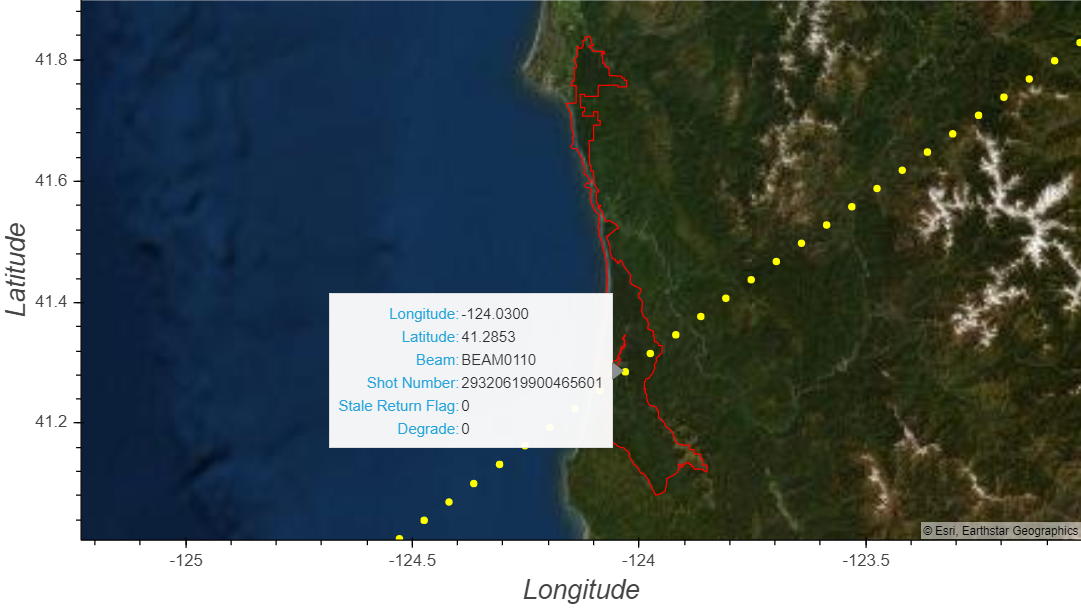
geoviews plots using *) with the point visual mapping function defined above in order to plot (1) the representative GEDI shots, (2) the region of interest, and (3) a basemap layer.¶# Call the function for plotting the GEDI points
gv.Polygons(redwoodNP['geometry']).opts(line_color='red', color=None) * pointVisual(latslons, vdims = vdims)
(HINT: find where the orbit intersects the west coast of the United States)

stale_return_flag and degrade mean?¶print(f"stale_return_flag: {gediL1B[b]['stale_return_flag'].attrs['description']}")
print(f"degrade: {gediL1B[b]['geolocation']['degrade'].attrs['description']}")
stale_return_flag: Indicates that a "stale" cue point from the coarse search algorithm is being used. degrade: Greater than zero if the shot occurs during a degrade period, zero otherwise.
2932: Orbit Number
06: Beam Number
199: Minor frame number (0-241)
00465601: Shot number within orbit
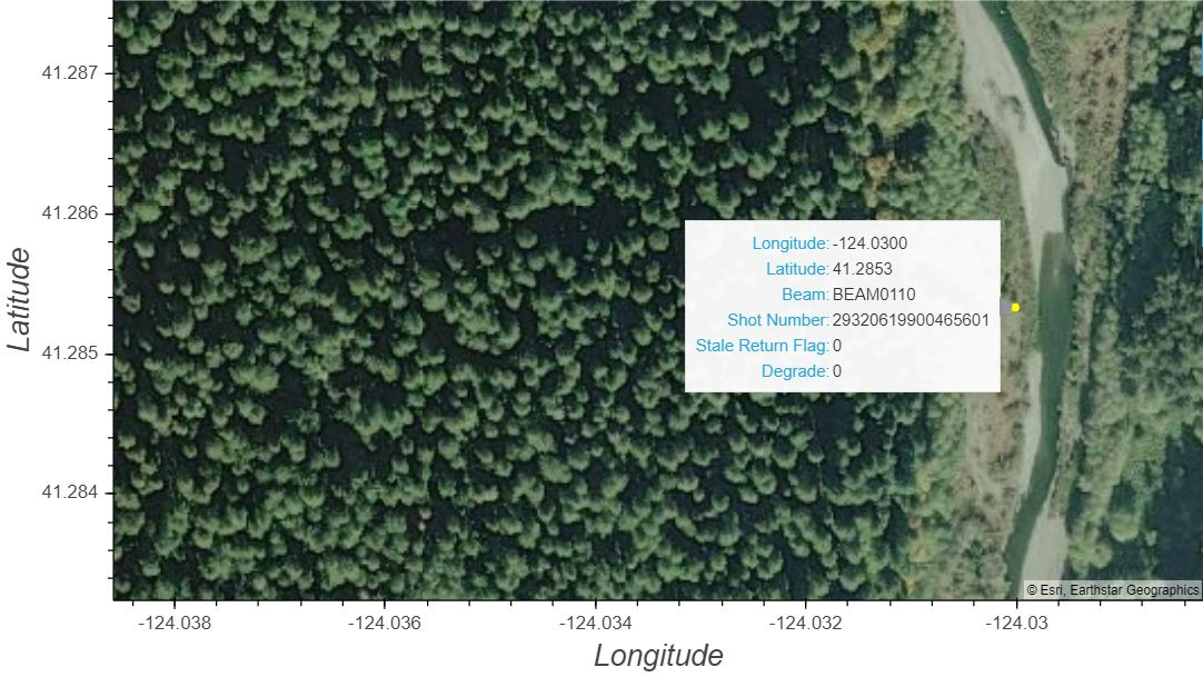
shot = 29320619900465601
index = np.where(gediL1B[f'{beamNames[0]}/shot_number'][()]==shot)[0][0] # Set the index for the shot identified above
index
465600
del latslons # No longer need the geodataframe used to visualize the full GEDI orbit
rx_sample_count and rx_sample_start_index to identify the location of the waveform that we are interested in visualizing and just extract those values.¶# From the SDS list, use list comprehension to find sample_count, sample_start_index, and rxwaveform
sdsCount = gediL1B[[g for g in gediSDS if g.endswith('/rx_sample_count') and beamNames[0] in g][0]]
sdsStart = gediL1B[[g for g in gediSDS if g.endswith('/rx_sample_start_index') and beamNames[0] in g][0]]
sdsWaveform = [g for g in gediSDS if g.endswith('/rxwaveform') and beamNames[0] in g][0]
print(f"rxwaveform is {gediL1B[sdsWaveform].attrs['description']}")
rxwaveform is The corrected receive (RX) waveforms. Use rx_sample_count and rx_sample_start_index to identify the location of each waveform.
print(f"rx_sample_count is {sdsCount.attrs['description']}")
print(f"rx_sample_start_index is {sdsStart.attrs['description']}")
rx_sample_count is The number of sample intervals (elements) in each RX waveform. rx_sample_start_index is The index in the rxwaveform dataset of the first element of each RX waveform. The indices start at 1.
rx_sample_count and rx_sample_start_index to identify the location of each waveform in rxwaveform.¶wfCount = sdsCount[index] # Number of samples in the waveform
wfStart = int(sdsStart[index] - 1) # Subtract one because python array indexing starts at 0 not 1
shot_number, and lat/lon location.¶wfShot = gediL1B[f'{beamNames[0]}/shot_number'][index]
wfLat = gediL1B[f'{beamNames[0]}/geolocation/latitude_bin0'][index]
wfLon = gediL1B[f'{beamNames[0]}/geolocation/longitude_bin0'][index]
print(f"The waveform located at: {str(wfLat)}, {str(wfLon)} (shot ID: {wfShot}, index {index}) is from beam {beamNames[0]} \
and is stored in rxwaveform beginning at index {wfStart} and ending at index {wfStart + wfCount}")
The waveform located at: 41.28533109208681, -124.0300090357876 (shot ID: 29320619900465601, index 465600) is from beam BEAM0110 and is stored in rxwaveform beginning at index 661152000 and ending at index 661152812
bin0 (the first elevation recorded) and lastbin or the last elevation recorded for that waveform.¶# Grab the elevation recorded at the start and end of the full waveform capture
zStart = gediL1B[f'{beamNames[0]}/geolocation/elevation_bin0'][index] # Height of the start of the rx window
zEnd = gediL1B[f'{beamNames[0]}/geolocation/elevation_lastbin'][index] # Height of the end of the rx window
print("{:,}".format(gediL1B[sdsWaveform].shape[0]))
1,391,172,580
# Retrieve the waveform sds layer using the sample start index and sample count information to slice the correct dimensions
waveform = gediL1B[sdsWaveform][wfStart: wfStart + wfCount]
# Find elevation difference from start to finish and divide into equal intervals based on sample_count
zStretch = np.add(zEnd, np.multiply(range(wfCount, 0, -1), ((zStart - zEnd) / int(wfCount))))
# match the waveform amplitude values with the elevation and convert to Pandas df
wvDF = pd.DataFrame({'Amplitude (DN)': waveform, 'Elevation (m)': zStretch})
wvDF
| Amplitude (DN) | Elevation (m) | |
|---|---|---|
| 0 | 226.009323 | 37.228645 |
| 1 | 225.360245 | 37.078965 |
| 2 | 225.373764 | 36.929286 |
| 3 | 226.165710 | 36.779607 |
| 4 | 227.480103 | 36.629927 |
| ... | ... | ... |
| 807 | 231.473923 | -83.562517 |
| 808 | 230.386932 | -83.712196 |
| 809 | 228.637512 | -83.861876 |
| 810 | 226.949661 | -84.011555 |
| 811 | 226.125153 | -84.161234 |
812 rows × 2 columns
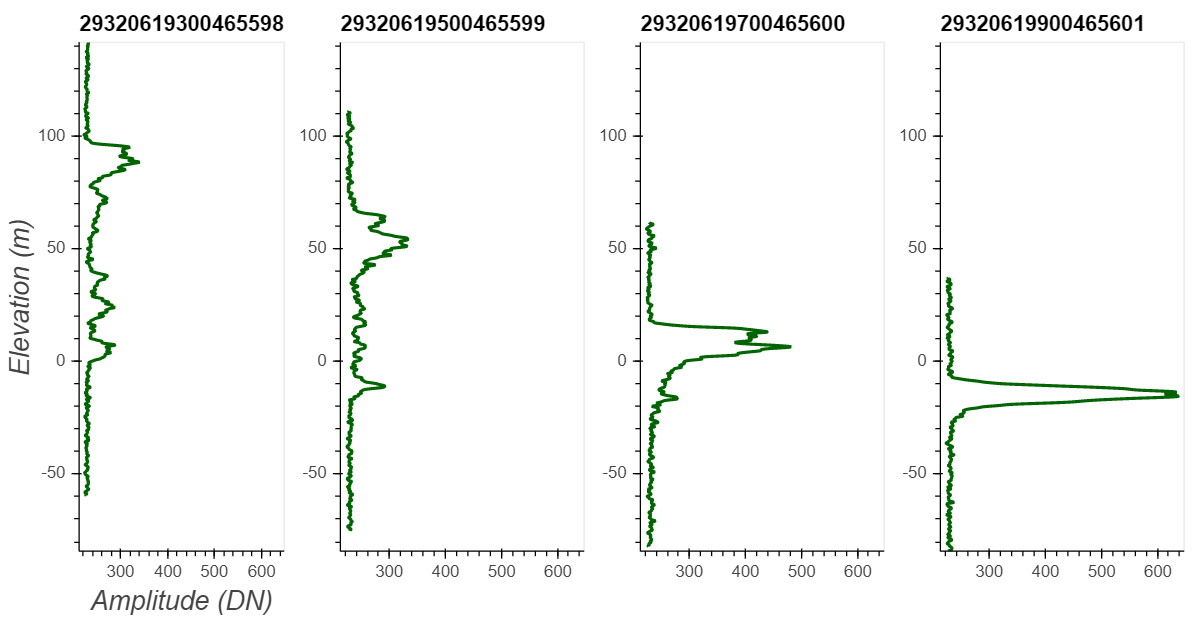
Holoviews python package (hv) to plot the waveform.¶hv.Curve(wvDF) # Basic line graph plotting the waveform
# Create a holoviews interactive Curve plot with additional parameters defining the plot aesthetics
wfVis = hv.Curve(wvDF).opts(color='darkgreen', tools=['hover'], height=500, width=400,
xlim=(np.min(waveform) - 10, np.max(waveform) + 10), ylim=(np.min(zStretch), np.max(zStretch)),
fontsize={'xticks':10, 'yticks':10,'xlabel':16, 'ylabel': 16, 'title':13}, line_width=2.5, title=f'{str(wfShot)}')
wfVis

latlons = {} # Set up a dictionary to hold multiple waveforms
latlons[wfShot] = Point(wfLon,wfLat) # Create shapely point and add to dictionary
# Retain waveform and quality layers to be exported later
latlonsWF = [waveform]
latlonsEL = [zStretch]
latlonsSRF = [gediL1B[f'{beamNames[0]}/stale_return_flag'][index]]
latlonsD = [gediL1B[f'{beamNames[0]}/geolocation/degrade'][index]]
# Define which observation to examine by selecting the three indexes prior to the one used above
index = 465597
# Use rx_sample_count and rx_sample_start_index to identify the location of each waveform
wfCount = sdsCount[index] # Number of samples in the waveform
wfStart = int(sdsStart[index] - 1) # Subtract 1, index starts at 0 not 1
wfShot = gediL1B[f'{beamNames[0]}/shot_number'][index] # Unique Shot Number
wfLat = gediL1B[f'{beamNames[0]}/geolocation/latitude_bin0'][index] # Latitude
wfLon = gediL1B[f'{beamNames[0]}/geolocation/longitude_bin0'][index] # Longitude
latlons[wfShot] = Point(wfLon,wfLat) # Create shapely point and add to dictionary
# Grab the elevation recorded at the start and end of the full waveform capture
zStart = gediL1B[f'{beamNames[0]}/geolocation/elevation_bin0'][index] # Height of the start of the rx window
zEnd = gediL1B[f'{beamNames[0]}/geolocation/elevation_lastbin'][index] # Height of the end of the rx window
# Retrieve the waveform sds layer using the sample start index and sample count information to slice the correct dimensions
waveform = gediL1B[sdsWaveform][wfStart: wfStart + wfCount]
# Find elevation difference from start to finish, divide into equal intervals
zStretch = np.add(zEnd, np.multiply(range(wfCount, 0, -1), ((zStart - zEnd) / int(wfCount))))
# match the waveform amplitude values with the elevation and convert to Pandas df
wvDF = pd.DataFrame({'Amplitude (DN)': waveform, 'Elevation (m)': zStretch})
# Append waveform and quality layers to be exported later
latlonsWF.append(waveform)
latlonsEL.append(zStretch)
latlonsSRF.append(gediL1B[f'{beamNames[0]}/stale_return_flag'][index])
latlonsD.append(gediL1B[f'{beamNames[0]}/geolocation/degrade'][index])
# Create a holoviews interactive Curve plot with additional parameters defining the plot aesthetics
visL1B1 = hv.Curve(wvDF).opts(color='darkgreen', tools=['hover'], height=500, width=400,
xlim=(np.min(waveform) - 10, np.max(waveform) + 10), ylim=(np.min(zStretch), np.max(zStretch)),
fontsize={'xticks':10, 'yticks':10,'xlabel':16, 'ylabel': 16, 'title':13}, line_width=2.5, title=f'{str(wfShot)}')
visL1B1
# Define which observation to examine by selecting the three indexes prior to the one used above
index = 465598
# Use rx_sample_count and rx_sample_start_index to identify the location of each waveform
wfCount = sdsCount[index] # Number of samples in the waveform
wfStart = int(sdsStart[index] - 1) # Subtract 1, index starts at 0 not 1
wfShot = gediL1B[f'{beamNames[0]}/shot_number'][index] # Unique Shot Number
wfLat = gediL1B[f'{beamNames[0]}/geolocation/latitude_bin0'][index] # Latitude
wfLon = gediL1B[f'{beamNames[0]}/geolocation/longitude_bin0'][index] # Longitude
latlons[wfShot] = Point(wfLon,wfLat) # Create shapely point and add to dictionary
# Grab the elevation recorded at the start and end of the full waveform capture
zStart = gediL1B[f'{beamNames[0]}/geolocation/elevation_bin0'][index] # Height of the start of the rx window
zEnd = gediL1B[f'{beamNames[0]}/geolocation/elevation_lastbin'][index] # Height of the end of the rx window
# Retrieve the waveform sds layer using the sample start index and sample count information to slice the correct dimensions
waveform = gediL1B[sdsWaveform][wfStart: wfStart + wfCount]
# Find elevation difference from start to finish, divide into equal intervals
zStretch = np.add(zEnd, np.multiply(range(wfCount, 0, -1), ((zStart - zEnd) / int(wfCount))))
# match the waveform amplitude values with the elevation and convert to Pandas df
wvDF = pd.DataFrame({'Amplitude (DN)': waveform, 'Elevation (m)': zStretch})
# Append waveform and quality layers to be exported later
latlonsWF.append(waveform)
latlonsEL.append(zStretch)
latlonsSRF.append(gediL1B[f'{beamNames[0]}/stale_return_flag'][index])
latlonsD.append(gediL1B[f'{beamNames[0]}/geolocation/degrade'][index])
# Create a holoviews interactive Curve plot with additional parameters defining the plot aesthetics
visL1B2 = hv.Curve(wvDF).opts(color='darkgreen', tools=['hover'], height=500, width=400,
xlim=(np.min(waveform) - 10, np.max(waveform) + 10), ylim=(np.min(zStretch), np.max(zStretch)),
fontsize={'xticks':10, 'yticks':10,'xlabel':16, 'ylabel': 16, 'title':13}, line_width=2.5, title=f'{str(wfShot)}')
visL1B2
# Define which observation to examine by selecting the three indexes prior to the one used above
index = 465599
# Use rx_sample_count and rx_sample_start_index to identify the location of each waveform
wfCount = sdsCount[index] # Number of samples in the waveform
wfStart = int(sdsStart[index] - 1) # Subtract 1, index starts at 0 not 1
wfShot = gediL1B[f'{beamNames[0]}/shot_number'][index] # Unique Shot Number
wfLat = gediL1B[f'{beamNames[0]}/geolocation/latitude_bin0'][index] # Latitude
wfLon = gediL1B[f'{beamNames[0]}/geolocation/longitude_bin0'][index] # Longitude
latlons[wfShot] = Point(wfLon,wfLat) # Create shapely point and add to dictionary
# Grab the elevation recorded at the start and end of the full waveform capture
zStart = gediL1B[f'{beamNames[0]}/geolocation/elevation_bin0'][index] # Height of the start of the rx window
zEnd = gediL1B[f'{beamNames[0]}/geolocation/elevation_lastbin'][index] # Height of the end of the rx window
# Retrieve the waveform sds layer using the sample start index and sample count information to slice the correct dimensions
waveform = gediL1B[sdsWaveform][wfStart: wfStart + wfCount]
# Find elevation difference from start to finish, divide into equal intervals
zStretch = np.add(zEnd, np.multiply(range(wfCount, 0, -1), ((zStart - zEnd) / int(wfCount))))
# match the waveform amplitude values with the elevation and convert to Pandas df
wvDF = pd.DataFrame({'Amplitude (DN)': waveform, 'Elevation (m)': zStretch})
# Append waveform and quality layers to be exported later
latlonsWF.append(waveform)
latlonsEL.append(zStretch)
latlonsSRF.append(gediL1B[f'{beamNames[0]}/stale_return_flag'][index])
latlonsD.append(gediL1B[f'{beamNames[0]}/geolocation/degrade'][index])
# Create a holoviews interactive Curve plot with additional parameters defining the plot aesthetics
visL1B3 = hv.Curve(wvDF).opts(color='darkgreen', tools=['hover'], height=500, width=400,
xlim=(np.min(waveform) - 10, np.max(waveform) + 10), ylim=(np.min(zStretch), np.max(zStretch)),
fontsize={'xticks':10, 'yticks':10,'xlabel':16, 'ylabel': 16, 'title':13}, line_width=2.5, title=f'{str(wfShot)}')
visL1B3
# The "+" symbol will plot multiple saved holoviews plots together
visL1B1.opts(width=240) + visL1B2.opts(width=240, labelled=[]) + visL1B3.opts(width=240, labelled=[]) + \
wfVis.opts(width=240, labelled=[])
# Convert dict to geodataframe
latlons = gp.GeoDataFrame({'Shot Number': list(latlons.keys()),'rxwaveform Amplitude (DN)': latlonsWF,
'rxwaveform Elevation (m)': latlonsEL, 'Stale Return Flag': latlonsSRF, 'Degrade': latlonsD,
'geometry': list(latlons.values())})
latlons['Shot Number'] = latlons['Shot Number'].astype(str) # Convert shot number from integer to string
vdims
['Beam', 'Shot Number', 'Stale Return Flag', 'Degrade']
# Create a list of geodataframe columns to be included as attributes in the output map
vdims = []
for f in latlons:
if f not in ['geometry']:
if 'rxwaveform' not in f:
vdims.append(f)
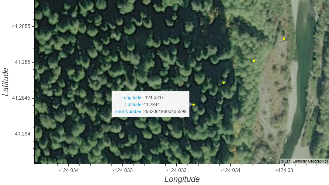
# Plot the geodataframe
gv.Polygons(redwoodNP['geometry']).opts(line_color='red', color=None) * pointVisual(latlons, vdims=vdims)


del wfVis, visL1B1, visL1B2, visL1B3, waveform, wvDF, zStretch, latlonsWF, latlonsEL, latlonsSRF, latlonsD
stale_return_flag is set to 1 (indicates that a "stale" cue point from the coarse search algorithm is being used) by defining those shots as nan.¶nan for that row.¶latlons = latlons.where(latlons['Stale Return Flag'].ne(1)) # Set any stale returns to NaN
degrade flag (Greater than zero if the shot occurs during a degrade period, zero otherwise).¶latlons = latlons.where(latlons['Degrade'].ne(1))
transectDF.¶latlons = latlons.dropna() # Drop all of the rows (shots) that did not pass the quality filtering above
print(f"Quality filtering complete, {len(latlons)} high quality shots remaining.")
Quality filtering complete, 4 high quality shots remaining.
del latlons
print(index)
465599
# Grab 50 points before and after the shot visualized above
start = index - 50
end = index + 50
transectIndex = np.arange(start, end, 1)
# Calculate along-track distance
distance = np.arange(0.0, len(transectIndex) * 60, 60) # GEDI Shots are spaced 60 m apart
holoviews Path() capabilities.¶# Create a list of tuples containing Shot number, and each waveform value at height (z)
wfList = []
for s, i in enumerate(transectIndex):
# Basic quality filtering from section 5
if gediL1B['BEAM0110/geolocation/degrade'][i] == 0 and gediL1B['BEAM0110/stale_return_flag'][i] == 0:
zStart = gediL1B['BEAM0110/geolocation/elevation_bin0'][i]
zEnd = gediL1B['BEAM0110/geolocation/elevation_lastbin'][i]
zCount = sdsCount[i]
zStretch = np.add(zEnd, np.multiply(range(zCount, 0, -1), ((zStart - zEnd) / int(zCount))))
waveform = gediL1B[sdsWaveform][sdsStart[i]: sdsStart[i] + zCount]
waves = []
for z, w in enumerate(waveform):
waves.append((distance[s], zStretch[z],w)) # Append Distance (x), waveform elevation (y) and waveform amplitude (z)
wfList.append(waves)
else:
print(f"Shot {s} did not pass quality filtering and will be excluded.")
import warnings
warnings.filterwarnings('ignore')
# Plot the waveform values for the transect with the waveform amplitude being plotted as the 'c' or colormap
l1bVis = hv.Path(wfList, vdims='Amplitude').options(color='Amplitude', clim=(200,405), cmap='Greens', line_width=20, width=950,
height=500, clabel='Amplitude',colorbar=True,
xlabel='Distance Along Transect (m)', ylabel='Elevation (m)',
fontsize={'title':16, 'xlabel':16, 'ylabel': 16, 'xticks':12, 'yticks':12,
'clabel':12, 'cticks':10}, colorbar_position='right',
title='GEDI L1B Waveforms across Redwood National Park: June 19, 2019')
l1bVis